NeurIPS 2022: Overcoming communication bottlenecks for decentralized training (2/2)

In our previous blog post, we introduced our work on scheduling foundation model training over heterogeneous networks. The algorithm assigns each tasklet of the training computation (a slice of the model and data)  to a set of GPUs connected by slow heterogeneous networks. We found that even when the network is 100 × slower, the end-to-end training throughput is only 1.7 ∼ 2.3 × slower. We now turn from scheduling (which is about globally laying out the computation to minimize communication) to the local problem of reducing communication between two nodes even more using compression.

In this post, we will talk about communication compression when communicating forward activations and backward gradients for fine-tuning foundation models in a decentralized environment to further unleash the potential of decentralized training. We introduce an algorithm, AQ-SGD that provides rigorous guarantees on SGD convergence. AQ-SGD is able to fine-tune large foundation models over slow networks (i.e., 500 Mbps) only 31% slower than no-compression in a fast datacenter network (i.e. 10 Gbps) in terms of end-to-end training performance.

Challenges for pipeline parallel communication relaxation

Significant research has studied communication compression for gradient synchronization in data parallelism with theoretical guarantees [1, 2, 3]. For example, gradient compression (e.g. quantization, sparsification, low-rank approximation, etc) is a popular approach, which significantly reduces communication volumes to accommodate the limitation of low network bandwidth. However, instead of simply aggregating gradients in data parallelism, foundation model training requires leveraging additional parallel strategies, such as pipeline parallelism — where GPUs also need to communicate the activations during the forward pass and the gradients on the activations during the backward pass. In this case, pipeline parallelism would take a large portion of the communication volumes — in a GPT3-1.3B fine-tuning example, given a pipeline partition of 8 stages, for one training iteration, the pipeline parallelism needs to communicate 15.03 GB of data while data parallelism needs to communicate 10.4 GB of data. In order to decrease the end-to-end communication, we have to compress both gradients and activations.

Although compressing the activations and corresponding gradients is easy to implement and looks natural at first glance, it turns out to be difficult to analyze: compressing the activations leads to a very different behavior compared with compressing the gradient — simply compressing these activations in a stochastically unbiased way will lead to biases in the gradient that cannot be measured easily or expressed in closed form. Without the theoretical guarantees, naive activation compression could lead to suboptimal training results for an aggressive compression rate, which limits the utilization of such methods in a real decentralized environment.

Activation compression by self-enforcing dynamics

One central problem we were trying to solve in this work is:

Can we design an algorithm for activation compression with rigorous theoretical guarantees on SGD convergence?

Toward this end, we propose a new approach named AQ-SGD: instead of directly compressing the activations, we compress the change of activations for the same training example across epochs. The intuition behind AQ-SGD is quite natural — when training stabilizes, the norm of the change of activations for the same training example across epochs becomes smaller. This decreases the maximal error caused by lossy compression which is related to the norm of the vectors that it compresses. This decrease in compression error will further make training converges more closely with the non-compression case.

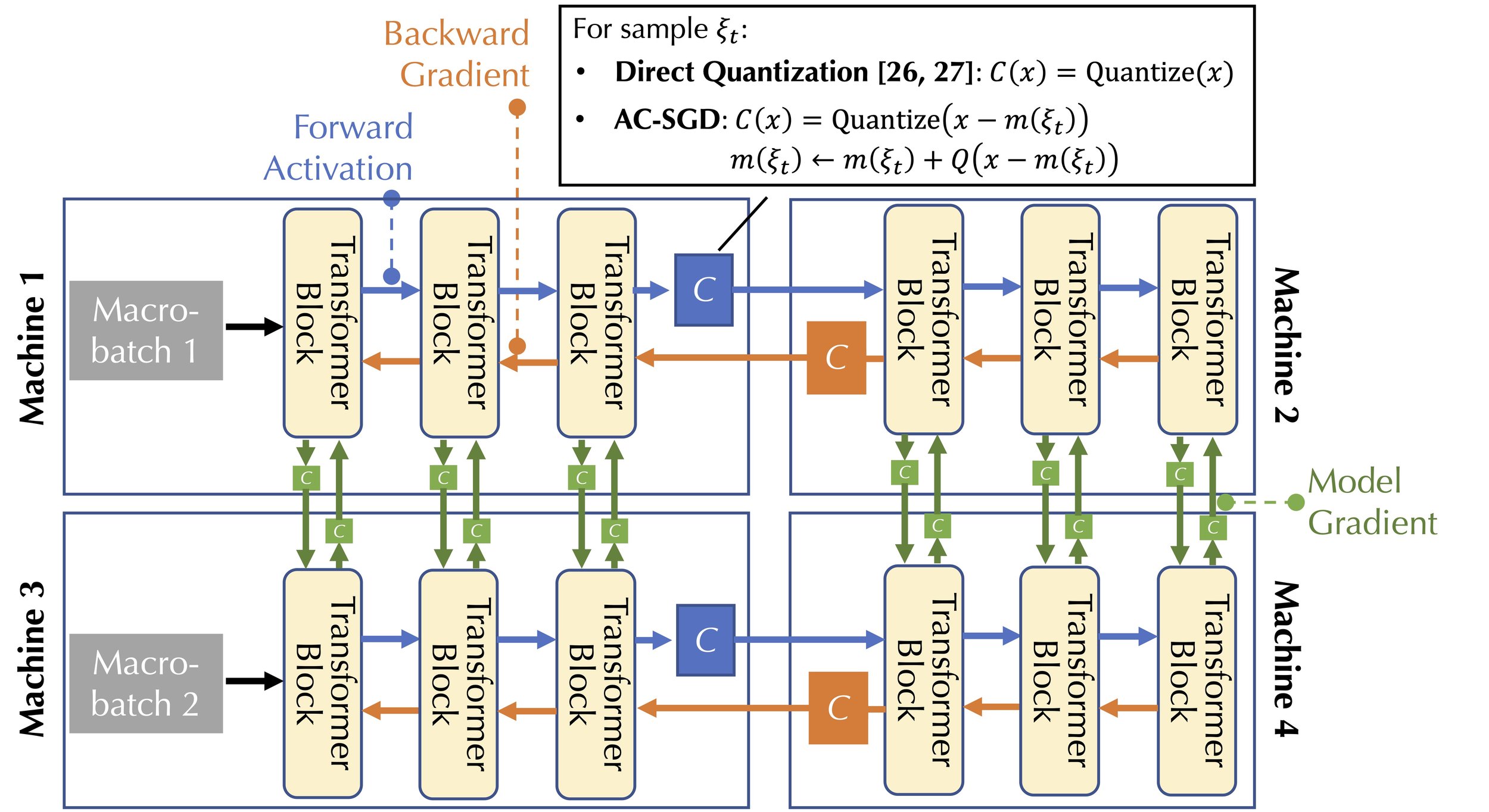
Figure 1 provides a visualization of the communication pattern of training foundation models. Within the scope of pipeline parallelism, in the forward pass, AQ-SGD will quantize the change of activations between epochs (noted by the blue compression block in Figure 1); in the backward pass, AQ-SGD will directly quantize the gradients of the corresponding activations (noted by the orange compression block in Figure 1). AQ-SGD can also be easily combined with gradient compression (noted by the green compression block in Figure 1) when needed.

For simplicity we state our algorithm based on pipeline with 2 stages, notice that it would be easy to extend the implementation and theoretical analysis to pipeline with more stages. Suppose two machines are utilized to optimize the following problem:

$$ \min_{x\in\mathbb{R}^d} \hspace{5mm} f(x) := \mathbb{E}_{\xi \sim \mathcal{D}} F ( b ( a(\xi, x^{(a)}), x^{(b)}) ) $$

where $F$ is a loss function, $a(-)$ and $b(-)$ represents two pipeline stages with the corresponding parameters $x^{(a)}$ and $x^{(b)}$. We formally describe the AQ-SGD algorithm between two machines that handles nearby

‍

Input:

   Learning rate: $\gamma$

   Model weights on predecessor Machine I: $x^{(a)}$

   Model weights on successor Machine II: $x^{(b)}$

   Quantization function: Q

Procedure:

   for t = 1, …, T do:

       // Forward pass:

       Randomly sample training data $\xi_t$;

       if $\xi_t$ is not seen before then:

           Set $m(\xi_t)$ ← $a(\xi_t, x_t^{(a)})$;

           Machine I sends $a(\xi_t, x_t^{(a)})$ to Machine II;

       else:

           Update $m(\xi_t) $ ← $m(\xi_t) + Q\big( a(\xi_t, x_{t}^{(a)}) - m(\xi_t)\big)$;

           Machine I sends  $Q\big( a(\xi_t, x_{t}^{(a)}) - m(\xi_t)\big)$ to Machine II;

       end if        

       // Backward pass:

       Update $x_{t+1}^{(b)}$← $x_{t}^{(b)} - \gamma \cdot \nabla_{x^{(b)}} (f\circ b)\vert_m$;

       Machine II sends $Q(\nabla_{a} (f\circ b)\vert_m)$ back to Machine I;

       Update $x_{t+1}^{(a)}$← $x_{t}^{(a)} - \gamma \cdot Q(\nabla_{a} (f\circ b)\vert_m) \cdot \nabla_{x^{(a)}} a$;

   end for

Concretely, in the forward pass, for each for iteration $t$ and the data sample $\xi_t$, if it is the first time that $\xi_t$ is sampled, Machine I communicates the full precision activations without any compression $m(\xi_t)=a(\xi_t, x_t^{(a)})$. Both machines will save $m(\xi_t)$ in a local buffer. If $\xi_t$ has been sampled in previous iterations, Machine I communicates a quantized version of $Q(a(\xi_t, x_t^{(a)}) - m(\xi_t))$, where $m(\xi_t)$ was the previous message, stored in the local buffer. Both machines then update this local buffer by $m(\xi_t)$←$m(\xi_t) + Q(a(\xi_t, x_t^{(a)}) - m(\xi_t))$.  On the other hand, in the backward pass, Machine II uses $m(\xi_t)$ as the forward activations, compute backward gradients, and communicate a quantized version of the backward gradient to Machine I. The idea behind this algorithm is simple — instead of quantizing the activations directly, we quantize the changes of activations for the same training example across epochs. Intuitively, since we are compressing the information in such a way that we compare with all the accumulated differences, this allows us to utilize the changes which appeared since the last time that we observed the current sample in an iterative way. On the other hand, as gradient updates are bounded by the learning rate — as long as we have a quantization method that keeps enough information about the signal, we can recursively build enough savings throughout the process. In particular, the more stability we have in the process, the smaller the changes in the model and the compression error gets, further strengthening the stability.

‍

Theoretical Analysis

We briefly state our theoretical analysis here, the complete proof can be found in our paper. Different from the previous theoretical analysis that makes assumptions that do not apply to neural networks with non-linear activation functions, e.g., an unbiased compression on activations leads to an unbiased error on the gradient, our main theorem shows that under standard assumptions, the convergence rate of AQ-SGD algorithm is $O(1/\sqrt{T})$ for non-convex objectives, the same as vanilla SGD.

Given the optimization problem:

$$ \min_{x\in\mathbb{R}^d} \hspace{5mm} f(x) := \mathbb{E}_{\xi \sim \mathcal{D}} F ( b ( a(\xi, x^{(a)}), x^{(b)}) ) $$

where $F$ is a loss function, $a(-)$ and $b(-)$ represents two pipeline stages with the corresponding parameters $x^{(a)}$ and $x^{(b)}$. We use the following standard assumptions:

• A1 Lipschitz assumption: We assume that $\nabla f$, $\nabla (f\circ b)$, and $a$ are $L_f$, $L_{f\circ b}$, and $\ell_a$-Lipschitz, respectively, recalling that a function $g$ is $L_g$-Lipschitz if
• $$ \| g(x) - g(y) \| \leq L_g \| x-y\|, \hspace{5mm} \forall x, \forall y. $$
• Furthermore, we assume that $a$ and $f\circ b$ have gradients bounded by $C_a$ and $C_{f\circ b}$, respectively, i.e., $\| \nabla a(x) \| \leq C_a$ and $\| \nabla (f\circ b) (x) \| \leq C_{f\circ b}$, $\forall x$.
• A2 SGD assumption: We assume that the stochastic gradient $g_\xi$ is unbiased, i.e. $\mathbb{E}_\xi [g_\xi (x)] = \nabla f(x), \forall $x, and with bounded variance, i.e. $\mathbb{E}_{\xi} \| g_\xi (x) - \nabla f(x) \|^2 \leq \sigma^2, \forall $x.

Theorem: suppose A1 and A2 hold, and consider an unbiased quantization function $Q(x)$ (e.g. randomized quantization: for any real number $z \in [a,b]$, with probability $\frac{b-z}{b-a}$ compress $z$ into $a$, and with probability $\frac{z-a}{b-a}$ compress $z$ into $b$), which satisfies that there exists $c_Q < \sqrt{1/2}$ such that $\mathbb{E} \| x-Q(x) \| \leq c_Q \|x\|$, for all $x$. Let $\gamma = \frac{1}{3(3L_f+C)\sqrt{T}}$ be the learning rate, where $C = \frac{4c_{Q} \ell_{a} (1+C_a) L_{f\circ b} N}{\sqrt{1-2c_{Q}^2}}$, $N$ is the number of training samples. Then after performing $T$ updates one will have:

$$ \frac{1}{T} \sum_{t\in [T]} \mathbb{E} \| \nabla f(x_t)\|^2 \lesssim \frac{(C+L_f)(f(x_1) - f^*)}{\sqrt{T}} + \frac{\sigma^2 + (c_{Q}C_aC_{f\circ b})^2}{\sqrt{T}}. $$

‍

Performance of AQ-SGD

In our empirical study, we find that: (1) AQ-SGD can tolerate very aggressive quantization on activations without compromising the quality of the model, which leads to 4.3× speed-up over the no-compression baseline; (2) AQ-SGD can be combined with state-of-the-art gradient compression techniques (e.g., QuantizedAdam), which achieves an 4.9× end-to-end speed-up.

Concretely, to evaluate AQ-SGD, we have the following setup of the experiments:

• Tasks: We consider both sequence classification and language modeling tasks with state-of-the-art foundation models. For sequence classification, we fine-tune a 1.5B parameter DeBERTa model on two datasets: QNLI and CoLA. For language modeling, we fine-tune the GPT2 model with 1.5B parameters on two datasets: WikiText2 and arXiv abstracts.
• Baselines: We compare with two baselines:
• FP32: All communications are in 32 bit floating point without any compression.
• DirectQ: Activations and backward gradients of the activations are directly quantized, following the protocol of [4, 5].

We summarize the interesting results in our experiments as below:

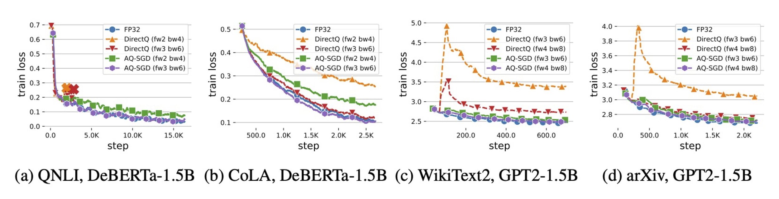
• Convergence: In Figure 2, we show the convergence behavior of different approaches. We learn that: FP32 converges fastest since it does not introduce any compression errors; DirectQ, under aggressive quantization, can converge to a significantly worse model, or even diverge — this is not surprising, given the biases on model gradients that direct quantization introduced. On the other hand, AQ-SGD converges almost as fast as FP32 in terms of number of training steps.

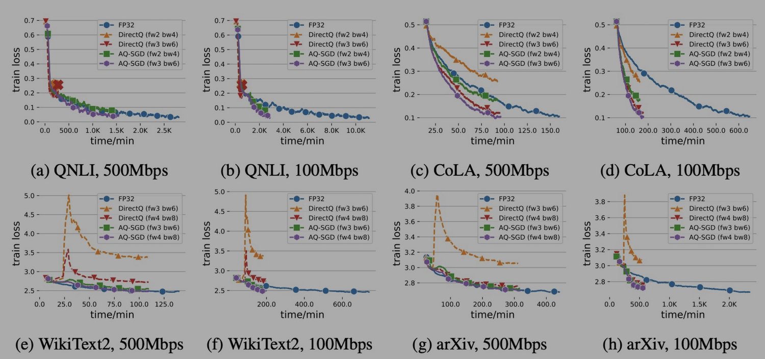
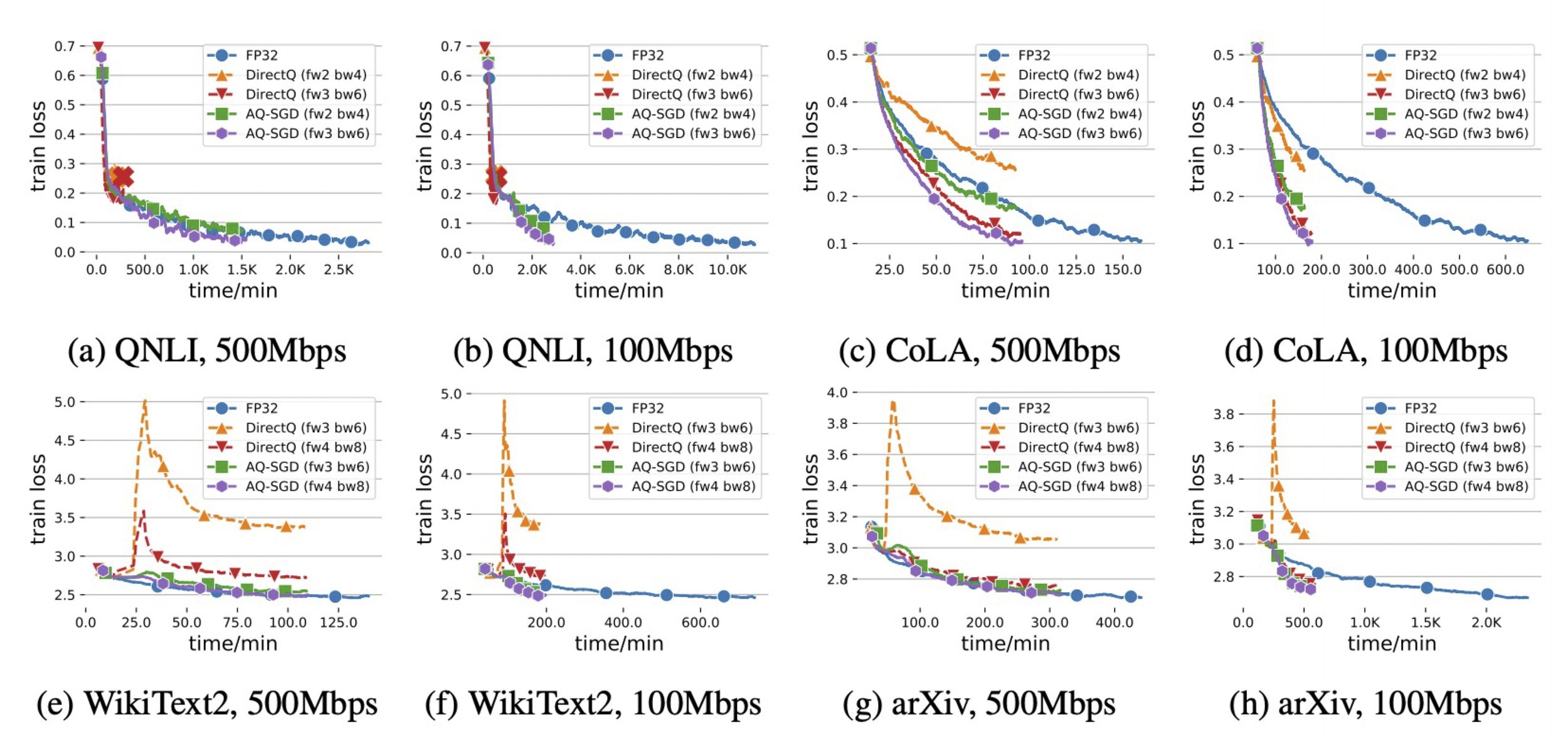
• Speedup in pipeline parallelism: In Figure 3, we show the end-to-end runtime of different approaches with the scope of pipeline parallelism under slow networks (500 Mbps and 100 Mbps — This is actually 100\times slower than the inter-machine connections within the data-center (10 Gbps)). We find that: AQ-SGD achieves a 4.3\times end-to-end speed-up comparing with that of FP32 (in terms of time to the same loss), illustrating the importance of communication compression in slow networks. Moreover, AQ-SGD in the decentralized slow network (i.e., 100 Mbps) is only 18% slower than no-compression in datacenter network (i.e. 10 Gbps). This shows the strong potential of decentralized training of foundation models.

• End-to-end communication compression: Lastly, we also verified that AQ-SGD can be combined with existing methods on gradient compression. Figure 4 shows that when combined with QuantizedAdam, AG-SGD can converge well, and leads to an up to 8.5\times throughput improvement comparing with the no-compression baseline. In this case, the end-to-end speedup is 4.9\times.

Future Explorations

Communication compression is another important aspect of decentralized learning, and we are super excited about what we learned in this paper. However, there are still many interesting open questions within this scope:

• Currently, we have shown the efficiency of AQ-SGD in the fine-tuning workflows, where it requires seeing each sample more than once. In the pre-train workflows, the training procedure might only go through the training set once, which makes it difficult to track the change of activations for the same sample during the training procedure. We might need to consider utilizing the activations from similar data samples that have been processed before.
• Another interesting question is that “Is it necessary to use fixed number of bits for quantization for each activation?” For example, can we dynamically determine the quantization bits given the heterogenous network bandwidths (e.g., [5, 6, 7])?
• Given a pre-defined precision level for communications, it is easy to apply the scheduling algorithm that we discussed in the previous post (we can just change the parameters corresponding to the amount of communications for different channels accordingly). But can we optimize these two dimensions, i.e., precision and scheduling, in a joint way?

These are very interesting future directions that we are exploring! Please let us know if you also find these questions to be interesting and we’d love to work together!