Even Better, Even Faster Quantized LLMs with QTIP

We’re excited to announce QTIP (Quantization with Trellises and Incoherence Processing), a new weight-only LLM post-training quantization method that achieves a state-of-the-art combination of quality and inference speed! QTIP compresses the weights of a model with trellis coded quantization, which achieves near-optimal distortion on a wide range of distributions. QTIP significantly improves over QuIP#’s [1] quality while being >3X faster than unquantized models.

How Does QTIP Work?

QTIP has two main components that enable both quality and speed. First, QTIP builds upon QuIP [2] and QuIP#’s incoherence processing framework. Specifically, QTIP uses the random Hadamard transform from QuIP#, which is both fast to multiply by and makes weight matrices approximately i.i.d. Gaussian. Then, to quantize these Gaussian matrices, QTIP uses trellis coded quantization (TCQ). Compared to vector quantization (VQ), which current SOTA methods such as QuIP# and AQLM [3] use, TCQ is able to achieve significantly lower distortion on i.i.d. Gaussian sources. This is in part due to TCQ’s linear cost in quantization dimension that lets it scale to much higher dimensions than VQ, which has exponential cost in dimension.

However, TCQ is not free. One of the main goals of weight-only quantization is to improve inference throughput in memory-bound settings such as small-batch inference. Therefore, it is important to be able to decode quantized weights as quickly as possible. Naively applying TCQ results in storage overheads that make fast decoding impossible. QTIP solves these problems by using the “bitshift trellis” and introducing a series of novel compute-based codes that trade memory for compute. These additions make TCQ fast to decode and thus practical for weight-only quantization.

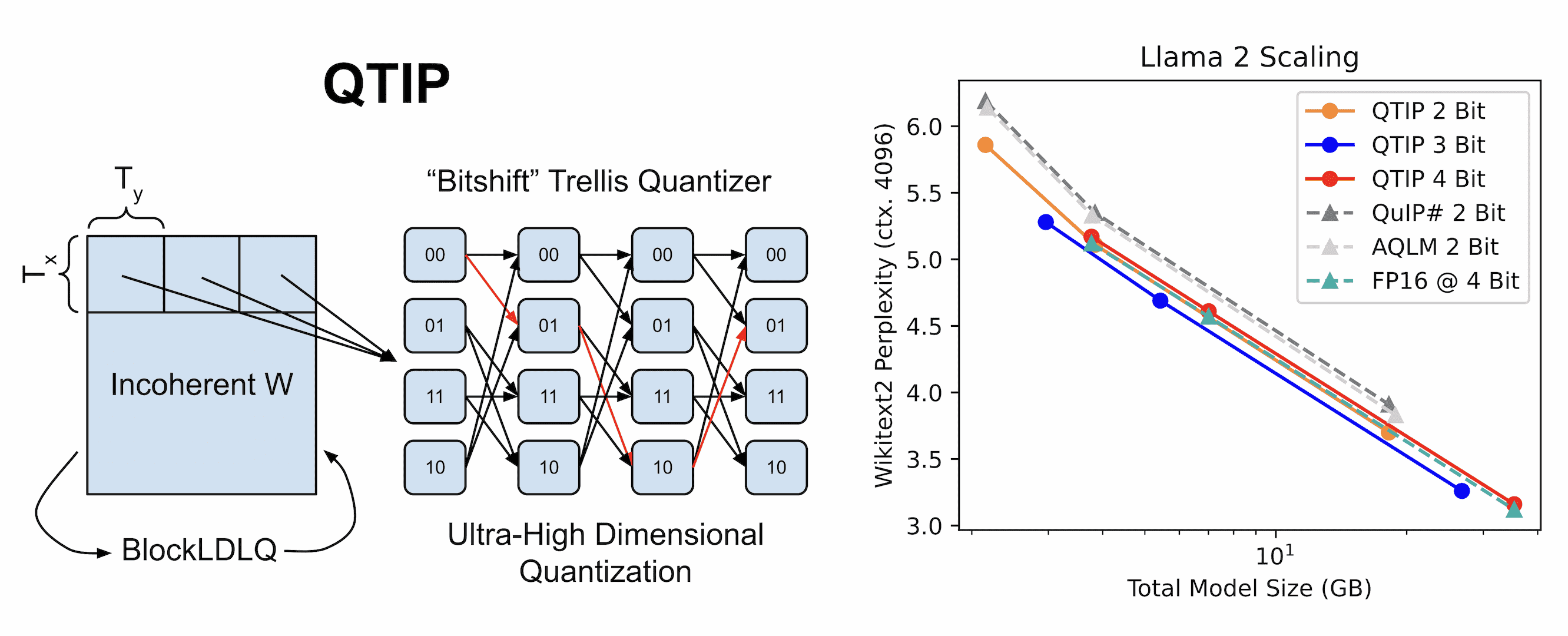
The rest of this blog post highlights key techniques and results from QTIP. As part of this release, we’ve put out prequantized QTIP models including Llama 3.1 405B Instruct and a codebase so you can quantize your own models. The full QTIP paper is available here and will appear at NeurIPS 2024 as a Spotlight.

Quantization for Faster Inference

LLM inference generally falls into two settings: compute-bound and memory-bound inference. In compute-bound settings, such as large-batch inference during prefill, inference speed is heavily dependent on the number of floating point operations (FLOPS) a machine can perform. Here, the cost of performing matrix multiplications dominates the cost of reading in model weights, so using a faster machine or a hardware-supported low precision datatype (e.g. FP8, INT4) is usually needed to get a meaningful speedup.

In memory-bound settings, such as small-batch decoding, inference speed is bound by how fast we can read weights in from memory. In these settings, the activations are usually much smaller than the weights and the cost of reading in weights dominates the cost of the matrix multiplication. Here, the memory bandwidth of the machine matters more than the number of FLOPs it can perform. For example, the NVIDIA H100 has around 3X the memory bandwidth of the NVIDIA RTX4090, so we can expect small-batch decoding to be around 3X faster on the H100 even though the RTX4090 can perform more FLOPS/s.

We can calculate an upper bound for small-batch inference throughput with

$$\text{Throughput (tok/s)} \leq \text{Batch Size (tok)} \times \frac{\text{Memory Bandwidth (GB/s)}}{\text{Model Size (GB)}}$$

If we want to make memory-bound inference go faster, our only realistic option is to make the model smaller. One way to do so is by quantizing each model parameter to use less information. Almost all LLMs today use 16 bits (e.g. BF16 or FP16) to store their parameters, which results in 2 bytes per parameter. However, not all 16 bits are necessary to get high quality predictions from models. Once trained, it is not hard to compress each parameter to 8 or even 4 bits without incurring significant model degradation. For example, most quantization methods today can produce near-lossless 4 bit Llama 2 models that achieve the same zeroshot performance as unquantized models.

{{custom-cta-1}}

Pushing Near-Lossless Quantization Below 4 Bits

Getting good quality and fast inference below 4 bits has been much harder. This is due to both having very little information to work with (a 2 bit model has 8 times less information than a 16 model) and needing to decode quickly to still get a throughput speedup. However, the QuIP line of works (QuIP, QuIP#, and now QTIP) have shown that it is indeed possible to achieve both good and fast models. 

Incoherence Processing

In QTIP, we follow existing works by quantizing each linear layer individually. Given a linear layer $y = Wx$, we wish to minimize the activation error over quantized weights $\hat W$

$$\mathbb{E}_{x\sim \mathcal{D}} \| (W-\hat W)x \|_F^2 = \mathbb{E}_{x \sim \mathcal{D}} tr(\Delta W xx^T \Delta W^T)$$

If we interpret $\mathbb{E}_{x\sim \mathcal{D}} [xx^T]$ as a proxy Hessian H, then this error becomes $\mathbb{E}_{x \sim \mathcal{D}}tr(\Delta W H \Delta W^T)$. In QuIP, the authors introduced the concept of “incoherence,” which measures the concentration of W and H by a factor $\mu$. If we use the LDLQ rounding algorithm (essentially GPTQ), then we can bound $\mathbb{E}_{x \sim \mathcal{D}}tr(\Delta W H \Delta W^T)$ by something $O(\mu^2 \sigma^2)$, where $\sigma$ is the error of the quantizer (e.g. a uniform scalar quantizer).

Now this might look complicated, but it essentially tells us that if we want to reduce the quantization error under LDLQ, we can either concentrate W and H to reduce $\mu$, use a better quantizer to reduce $\sigma$, or do both. To do the former, QuIP introduced the concept of “Incoherence Processing” (IP), which conjugates W and H with random orthogonal matrices to reduce $\mu$. With an appropriately chosen class of random orthogonal matrices, QuIP enabled the first usable 2 bit LLMs. 

QuIP achieved its groundbreaking results with a specially constructed class of random orthogonal matrices and a uniform scalar quantizer. As it turns out, both were pretty suboptimal. QuIP# improved upon QuIP by introducing the random Hadamard transform (RHT) and vector quantization (VQ). QuIP’s random orthogonal matrices required $O(n\sqrt{n})$ time to multiply by – in contrast, the RHT requires $O(n \log n)$ time. Furthermore, the RHT achieved better theoretical and empirical concentration, producing essentially i.i.d Gaussian weight matrices.

This Gaussian shaping meant that we could go from scalar quantization to vector quantization. In scalar quantization, each number is quantized individually. In vector quantization, a group of numbers (a vector) is quantized together to a codebook of entries. This allows us to shape the codebook to the vector’s joint distribution and better utilize information. The image below from GPTVQ [4] illustrates this for a 2D Gaussian distribution. No matter which scalar quantizer you use (left and center), the “corners” of the effective codebook will have poor information utilization. In contrast, with 2D VQ, we can shape the codebook to match the source distribution. QuIP# introduced a special 8D vector quantizer based on the E8 lattice. This significantly reduced  over QuIP’s scalar quantizer and enabled the first high-quality 2 bit LLMs that were also even faster than QuIP’s models.

Better Quantization with Trellis Coding

Much of VQ’s advantage of SQ comes from shaping and dimensionality. However, scaling VQ is expensive. Both encoding to and decoding from an unstructured VQ codebook cost exponential space and time in dimension and bitrate since the number of code points in the codebook grows exponentially. That means that a 16D vector quantizer would be 256X more expensive to decode from than QuIP#, limiting how high of a dimension we can reach with VQ. In QTIP, we solve this problem by instead using trellis coded quantization, which has linear cost in dimension. With TCQ, we can quantize arbitrary long sequences and achieve significantly lower distortion than VQ. In fact, TCQ reduces the distortion gap between QuIP# and an optimal 2 bit quantizer by over 3X!

The main insight behind TCQ is to make quantization stateful. In VQ, each group of weights is quantized to one entry in a codebook. In trellis quantization, a sequence of numbers is quantized according to a directed graph G, which is “unrolled” to form a trellis. Specifically, for K-bit TCQ, each node in G is assigned a high-precision value (e.g. a FP16 number) and has $2^K$ outgoing edges. The set of representable sequences is the set of walks on G, where a sequence is given by the concatenation of node values in the walk. This might be a bit confusing, but essentially each new value being quantized gets assigned to an edge that chooses which node to go to next. Since each node has $2^K$ outgoing edges, we only need K bits to store which edge to take, making this K bit quantization.

The diagram above shows an example for quantizing a sequence of 6 numbers (0.54, 0.03, 0.72, 0.19, 0.26, 0.89) to a 1 bit trellis with 4 nodes. Since K=1, each node has $2^1 = 2$ outgoing edges. Node 0 (following the binary numbering in the figure) has value 0.5, node 1 has value 0.1, node 2 has value 0.8, and node 3 has value 0.3. The closest (by MSE) representable sequence consists of nodes 0, 1, 2, 1, 3, and 2, and only requires storing the initial node (0) and whether we took the top (T) or bottom (B) edge. This means that the quantized sequence can be stored as (0, B, B, T, B, B), which takes 7 bits since it takes 2 bits to store node 0 (G has 4 nodes). Apart from storing the initial node, each additional number indeed only requires 1 bit to store, as desired.

In practice, we want the number of nodes to be much higher than the bitrate (edges per node). More nodes means more node values that form a larger “codebook” that better models the source distribution of the input sequence. This lets us increase the probability that we can find a walk that is close to the original sequence and gives low quantization distortion. To actually find the optimal walk under some additive error metric, we can use the Viterbi algorithm. The Viterbi algorithm uses dynamic programming to track the best sequence ending at each node for each number in an input sequence. Assuming G has $2^L$ nodes and we are quantizing a length-T sequence, the Viterbi algorithm runs in $O(2^L T)$. This means that TCQ scales linearly with dimension (T), letting us hit arbitrarily high dimensions.

Choosing a Fast Trellis

So far, TCQ sounds pretty good. It achieves lower distortion than VQ, scales better, and we can always grow some plants on the trellis if it fails. Have you ever tried growing plants on a vector? Yeah, neither have we. However, TCQ isn’t perfect. Our goal is still fast decoding for fast inference, and it can be difficult to decode trellis-coded sequences quickly. To decode an encoded sequence, we need to know G and the codebook. This means we need to store $2^{LK} L$ bits information for G’s structure ($2^L$ nodes, $2^K$ edges per node, and L bits per edge) and $2^L 16$ bits for a 16 bit codebook. Furthermore, because an encoded entry can depend on all the previous entries in the sequence, we can’t decode a sequence in parallel. This is problematic since GPUs are highly parallel; we want to take advantage of this property to ensure fast inference.

We can solve both this parallelism problem and needing to store the graph structure with the “bitshift trellis.” The bitshift trellis was introduced by Mao and Gray as part of the “random permutation trellis coder” [5]. In the bitshift trellis, node i has an edge to node j if the lower L-K bits of the binary representation of i are the same as the upper L-K bits of the binary representation of j. Formally, node i has an edge to node j if $\lfloor j/2^K \rfloor = (i \mod 2^{L-K})$ . For example, in the example below, L=12 and K = 2. Node 2856 has an edge to node 3234 since the bottom 10 bits of bin(2856) are the same as the top 10 bits of bin(3234).

With the bitshift trellis, we no longer need to store G’s structure. Given a bitstream containing an encoded sequence, we can simply get from one node to the next by shifting by K bits (hence the name bitshift). Furthermore, since each encoded node is defined by a length-L window in this bitstream, we can decode this sequence in parallel. That is, we can start decoding from any place in the bitstream since any encoded number is only dependent on the last L bits. 

Designing Fast Codebooks

The bitshift trellis only tells us what G’s structure looks like – it doesn’t say anything about what values each node (the codebook) should take. Since we know that incoherence processing with the RHT produces approximately Gaussian weights, it makes sense to make the codebook contain Gaussian-distributed values. However, we cannot simply store an entire codebook as a $2^L 16$ bit lookup table (LUT) if we want to perform fast decoding on GPUs, which we do. 

To better understand why, let’s look at what happens when we decode a bitshift trellis-encoded sequence. For each element we decode, we read in a L bit window containing its node ID. This L bit number is used to index into the codebook to read out a decoded value. Since the input sequence to the quantizer is approximately i.i.d. Gaussian (from incoherence processing), we are essentially performing lots of random reads from the codebook. This means that the entire codebook must fit in a GPU’s L1 cache after being duplicated 32 (NVIDIA) or 64 (AMD) times to avoid bank conflicts. On something like the H100, we can realistically have a 4KB LUT before running out of L1 cache and bottlenecking decoding. This works out to L=8 (256 states), which is not very high. Although L=8 will already give lower distortion than vector quantization, we want L to be as high as possible for maximum quality.

To solve this problem, QTIP introduces a series of compute-based codes that take the L bit window and compute out a pseudorandom Gaussian number. These codes use as few as 3 ALU instructions to generate one number, making them efficient on hardware. These codes are also designed to avoid correlations caused by the bitshift trellis. Since adjacent nodes in the bitshift trellis share L-K bits, a poorly designed code can have “missing” entries in the set of representable points. The figure below shows this visually by plotting the set of representable pairwise adjacent values under the bitshift trellis. The leftmost plot shows a poorly designed code with poor coverage of a Gaussian distribution (the rightmost plot). The center two codes are QTIP’s compute-only codes, 1MAD and 3INST. Both 1MAD and 3INST require no lookups at all and do a good job of emulating a Gaussian distribution.

The results we present later mainly use the “HYB” code that computes a pseudorandom index and performs a lookup into a small codebook. Since modern GPUs have enough L1 cache to handle small lookups, we can take advantage of this by having a hybrid compute-lookup code. The image below shows the details of HYB. For more details on 1MAD and 3INST, see the paper.

Results

Putting everything together, now it’s time to see if trellis coded quantization is actually better than vector quantization when quantizing real-world models. To test this, we used the bitshift trellis and QTIP’s computed codes as drop-in replacements for QuIP#’s vector quantizer. 

For the standard Llama 1 and 2 test suite of models, QTIP strongly outperforms QuIP#, AQLM, and GPTVQ – three vector-quantization-based methods. This shows that even after recovery-based fine-tuning (RFT), which fine-tunes the quantized model to recover the original model, TCQ’s improvements over VQ still hold up.

This difference is so large that QTIP without RFT is able to match or exceed QuIP# and AQLM with RFT.

On the more recent Llama 3.1 family of models, which have been reported to be harder to quantize than Llama 2, we once again see that QTIP is able to achieve strong results at 4 bits and below. On zeroshot tasks, QTIP models have minimal degradation down to 2-3 bits. This is especially impressive for Llama 3.1 405B, which doesn’t even fit on a single 8xH100 node without some form of compression. In contrast, QTIP’s 2 Bit Llama 3.1 405B is able to fit on 2 NVIDIA H100s.

Decoding Speed

Finally, we ask the 100 billion dollar question: is TCQ worth it and is QTIP actually practical? To answer this, we measured the decoding throughput for the HYB code for batch size 1 inference on an NVIDIA RTX6000 Ada GPU. At both tested model sizes, QTIP achieves the same impressive inference speeds as QuIP#, making QTIP’s quality improvements essentially free.

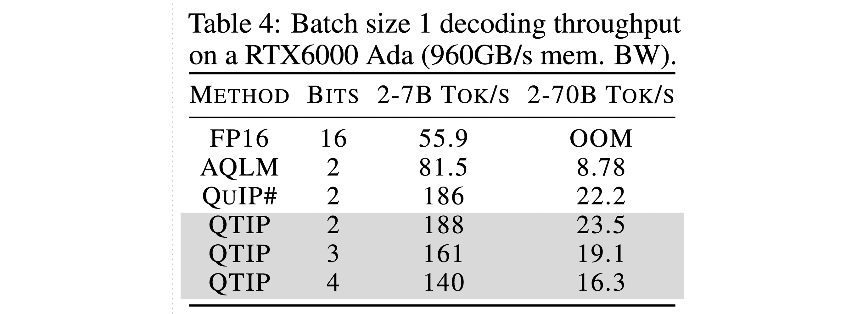
Furthermore, due to QTIP’s flexibility – there are many ways to generate pseudorandom Gaussians with very few instructions – QTIP can be fast on a wide class of hardware. Our paper describes 3 codes that range from compute-only codes (no cache required) to hybrid compute-lookup codes tuned for modern GPUs. However, there is nothing stopping you from developing your own code for using QTIP on your own hardware!

Using QTIP

Like the actual thing, you probably shouldn’t stick QTIP in your ear. QTIP was designed to accelerate memory-bound inference, so it won’t help if your inference is compute-bound. For compute-bound settings, you should consider using weight-activation quantized models that can take advantage of hardware-supported low-precision datatypes. Alternatively, you can use Together AI’s high-performance APIs, which are probably way easier to call. 

Finally, as part of this release, we’ve put out prequantized QTIP models including Llama 3.1 405B Instruct and a codebase so you can quantize your own models. The full QTIP paper is available here and will appear at NeurIPS 2024 as a Spotlight.

References

1. QuIP#: Even Better LLM Quantization with Hadamard Incoherence and Lattice Codebooks. Albert Tseng*, Jerry Chee*, Qingyao Sun, Volodymyr Kuleshov, Christopher De Sa. ICML 2024.
2. QuIP: 2-Bit Quantization of Large Language Models With Guarantees. Jerry Chee, Yaohui Cai, Volodymyr Kuleshov, Christopher De Sa. NeurIPS 2023.
3. Extreme Compression of Large Language Models via Additive Quantization. Vage Egiazarian*, Andrei Panferov*, Denis Kuznedelev, Elias Frantar, Artem Babenko, Dan Alistarh. ICML 2024.
4. GPTVQ: The Blessing of Dimensionality for LLM Quantization. Mart Van Baalen*, Andrey Kuzmin*, et al. ICML 2024 ES-FoMo II Workshop.
5. Rate-Constrained Simulation and Source Coding IID Sources. Mark Z. Mao, Robert M. Gray, Tamas Linder. IEEE Transactions on Information Theory.